April 10, 2026
Table of Contents
I was building a document search system when something odd happened. The retrieval scores looked fine - cosine similarities in the 0.85+ range, top-5 results all semantically relevant. But the LLM kept generating wrong answers. Not hallucinations - it was faithfully summarizing the retrieved documents. The documents themselves were wrong.
The query was about a specific row in a financial table. The correct page existed in the corpus, but the ingestion pipeline had split the table across two chunks, garbled two column headers via OCR, and the embedding model had compressed what was left into a single vector that happened to be closer to a different table with similar vocabulary. Every step in the pipeline worked as designed. The pipeline itself was the problem.
This is the reality of most enterprise RAG (Retrieval Augmented Generation) systems. The failure is not in any single step - it compounds across the entire pipeline, from how documents are parsed, to how they are vectorized, to how they are retrieved. And it is almost invisible because the similarity scores look perfectly reasonable while the system quietly serves the wrong context.
I benchmarked a fundamentally different approach - multi-vector multimodal embeddings that skip the entire parse-chunk-embed chain - testing 16 configurations to map the quality trade-offs. The results changed how I think about document representation for search.
Where Does the Traditional RAG Pipeline Break?
The standard RAG pipeline has three compounding bottleneck layers. Fixing only one does not solve the problem because the others continue to degrade quality:
Bottleneck 1: Document Ingestion
Before any embedding happens, documents go through a chain of preprocessing steps - layout detection, OCR, table extraction, chunking, and sometimes captioning. The ColPali paper (ICLR 2025) measured this pipeline at 7.22 seconds per page and found that optimizing the ingestion pipeline yielded more improvement than switching to a better embedding model. The bottleneck was not the model - it was the preprocessing chain.
Each step in this chain introduces errors that compound downstream. Layout detection misclassifies a chart as text. OCR garbles table cell boundaries. Chunking splits a table across two chunks. By the time text reaches the embedding model, it may barely resemble the original document.
Bottleneck 2: Vectorization
Even with perfect text extraction, the standard embedding step compresses an entire document chunk into a single vector - typically 768 or 1024 dimensions. A paragraph about quarterly revenue, a footnote about methodology, and a table header all collapse into one point in vector space. Research consistently shows this lossy compression forces multi-faceted information into a single representation, losing the fine-grained semantic nuances that matter for precise retrieval.
Bottleneck 3: Retrieval
The final layer of failure is the retrieval mechanism itself. Standard cosine similarity computes a single number between a query vector and a document vector. This conflates semantic similarity with relevance - two concepts that sound similar but are fundamentally different. A document about “Q2 revenue growth in APAC” and a document about “Q2 revenue decline in Europe” will score similarly against a query about “Q2 revenue in APAC” because the vocabulary overlaps. The retrieval step has no mechanism to distinguish the nuance.
| Pipeline Layer | What Breaks | Why It’s Hard to Fix in Isolation |
|---|---|---|
| Ingestion | OCR errors, lost tables/charts, broken layouts | Even perfect OCR cannot reconstruct visual semantics |
| Vectorization | Lossy single-vector compression | More dimensions help marginally; the representation paradigm is the limit |
| Retrieval | Similarity != relevance, no fine-grained matching | Better similarity metrics cannot compensate for information lost upstream |
The multi-vector multimodal approach does not incrementally improve one layer. It replaces the entire pipeline with a fundamentally different architecture - an example of the kind of paradigm shift that separates genuine transformation from incremental tooling updates.
How Does Multi-Vector Late Interaction Actually Work?
Instead of the parse-chunk-embed-retrieve chain, multi-vector models take a document page as an image and produce one embedding per image patch (or token). A document with 1024 patches generates 1024 vectors, each capturing the semantic content of a specific region - a table cell, a chart label, a paragraph, a heading.
The retrieval mechanism - called late interaction - works differently from cosine similarity:
flowchart TD
    Q["Query: 'What is the Q3 revenue?'"] --> QT["Tokenize into N query vectors"]
    D["Document Page (as image)"] --> DP["Generate M patch vectors
1 vector per image region"]
    QT --> MS["MaxSim Scoring:
Each query token finds its
best-matching document patch"]
    DP --> MS
    MS --> SUM["Sum all best-match scores
= Fine-grained relevance"]
This is the MaxSim operator from ColBERT (Khattab & Zaharia, 2020): for each query token, find the maximum dot product with any document token, then sum across all query tokens. The key insight is that each query term independently finds its best match in the document. When a query asks “What is the Q3 revenue?”, the system identifies the specific table cell where Q3 revenue appears and scores it directly - rather than asking whether the entire document is “about” revenue.
This fixes all three bottlenecks simultaneously:
| Bottleneck | Traditional Approach | Multi-Vector Approach |
|---|---|---|
| Ingestion | Parse → OCR → chunk → caption (7.22s/page) | Render page as image → embed directly (0.39s/page) |
| Vectorization | 1 vector per chunk (~8.6 KB) | 1 vector per patch, preserving spatial/semantic detail |
| Retrieval | Cosine similarity (coarse, single score) | MaxSim late interaction (fine-grained, per-token matching) |
The Architecture Behind It
The core idea is deceptively simple: take a Vision Language Model (VLM) - the same type of model that can describe images and answer questions about them - and repurpose its internal representations for search instead of generation.
The ColPali model (published at ICLR 2025) was the breakthrough that proved this works at scale. It takes PaliGemma-3B, a VLM that already understands both text and images, and adds a projection layer that maps each of the model’s output embeddings (whether from text tokens or image patches) into a shared 128-dimensional vector space. The late interaction score is then computed between projected query token embeddings and projected document patch embeddings - giving us a fine-grained relevance signal without ever extracting text from the document.
On the original ViDoRe benchmark, ColPali achieved 81.3 nDCG@5 - compared to 67.0 for the best traditional pipeline (Unstructured + BGE-M3 with captioning). The gap was largest on visually complex documents: infographics (+14.4), figures (+22.6), and tables (+7.0). Even on text-heavy documents, ColPali outperformed traditional approaches across all evaluated domains and languages.
The field has since evolved rapidly. The latest benchmark - ViDoRe v3 (January 2026) - is now the industry standard, covering 10 enterprise-relevant document corpora across 6 languages with ~26,000 pages and 3,099 human-verified queries. It is integrated into the MTEB leaderboard for standardized evaluation. The current top model on ViDoRe v3 is NVIDIA’s nemotron-colembed-vl-8b-v2 at 63.42 nDCG@10, followed by several ColQwen variants. These scores are lower than the original ViDoRe because v3 is deliberately harder - built on 12,000 man-hours of human annotations across enterprise domains like finance, pharmaceuticals, and industrial documents.
ColNomic - the model I benchmarked - extends the ColPali paradigm to the Nomic Embed ecosystem, fine-tuning from Qwen2.5-VL in 3B and 7B variants with additional training innovations like same-source sampling for harder in-batch negatives. The 7B variant scores 57.33 nDCG@10 on ViDoRe v3 (ranked 8th), and is released under Apache 2.0 - making it a practical open-source option for enterprise deployment.
What Did the Benchmark Reveal About Quality?
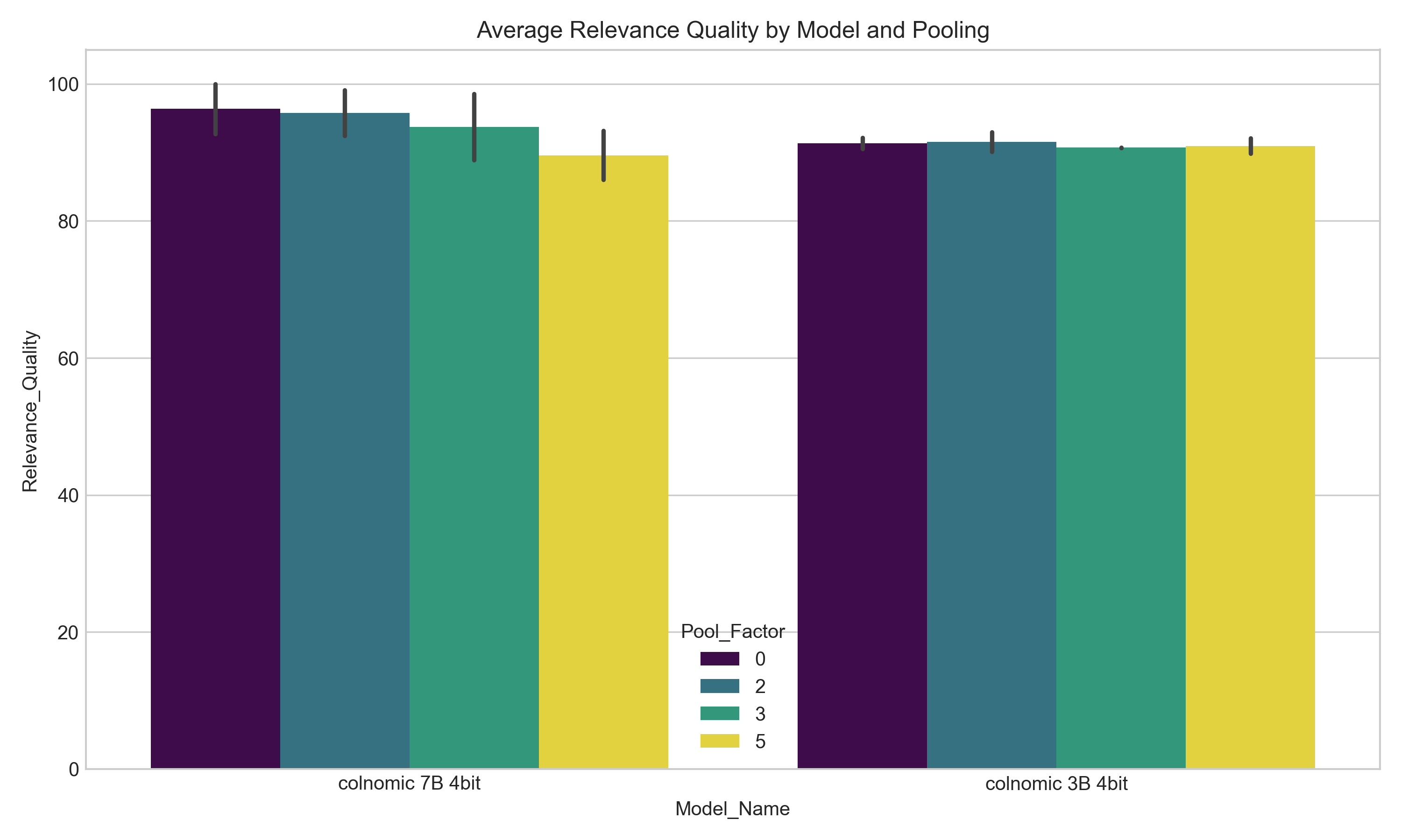
To understand the practical trade-offs, I set up a structured benchmark using ColNomic 7B and 3B (both 4-bit quantized) across 16 configurations. I varied three parameters: model size, image resolution (1920x1080 vs 448x448), and token pooling factor (0, 2, 3, 5). Token pooling is a compression technique from the ColPali paper that merges similar patch vectors hierarchically - reducing the number of vectors without discarding the multi-vector paradigm.
I ran each configuration against 9 retrieval queries on 4 mixed-modality files (text and images), measuring relevance quality via MaxSim scoring. The goal was not to crown a winner, but to map the quality-speed frontier so engineering teams can make informed decisions for their specific constraints.
Three Key Quality Findings
1. Token pooling at factor 2 is the universal sweet spot. Across both models and resolutions, pooling by a factor of 2 delivered less than 1% quality degradation while halving the number of stored vectors. The ColPali paper reported the same - pool factor 3 retained 97.8% of ViDoRe performance while reducing vectors by 66.7%. For any production deployment, pool factor 2 should be the starting default.
2. Larger models benefit significantly from higher resolution; smaller models do not. The 7B model showed a clear quality jump from 448x448 to 1920x1080 resolution (92.7% → 100%). The 3B model showed almost no improvement (92.2% → 90.5% - actually slightly worse). The smaller model lacks sufficient capacity to leverage additional visual detail. Throwing more pixels at a smaller model wastes compute.
3. Model capacity matters more than aggressive compression. The 7B model at pool factor 5 (aggressive compression) still scored 93.2% quality - higher than the 3B model with no compression at high resolution (90.5%). When quality is the primary concern, investing in a larger model with moderate compression outperforms a smaller model with maximum fidelity.
The Pareto Frontier
Out of 16 configurations tested, 9 are Pareto-optimal - meaning no other configuration is strictly better on all dimensions. This tells us there is no single “best” configuration; the right choice depends entirely on what you are optimizing for.
| Configuration | Quality | Processing Time |
|---|---|---|
| 7B, High-res, No pooling | 100% | 3.1s |
| 7B, High-res, Pool:2 | 99.1% | 3.3s |
| 7B, High-res, Pool:3 | 98.6% | 3.3s |
| 3B, Low-res, Pool:2 | 93.0% | 1.1s |
| 3B, Low-res, No pooling | 92.2% | 1.0s |
| 3B, Low-res, Pool:5 | 89.8% | 1.2s |
How Should You Choose Your Approach?
Rather than recommending specific models or configuration numbers - which will be outdated within months as new models release - here is a decision framework based on the architectural priorities that remain stable:
| Your Priority | Approach | Why |
|---|---|---|
| Maximum retrieval quality (regulated industries, legal, financial) | Largest available multi-vector model + moderate token pooling (factor 2-3) + highest resolution your infrastructure supports | Larger models extract more nuance from visual detail; moderate pooling has negligible quality cost |
| Low latency (real-time search, user-facing Q&A) | Smallest multi-vector model + low resolution + moderate pooling | Sub-second processing is achievable; quality remains above 90% for most document types |
| Scale to millions of documents | Two-stage pipeline: fast lightweight retrieval for candidate selection → multi-vector re-ranking on top-K results | The ColPali paper explicitly recommends this hybrid approach; combines broad recall with precise re-ranking |
| Mixed document corpus (some visual, some text-only) | Hybrid architecture: multi-vector for visually rich documents + traditional embeddings for clean text | Apply the right tool for the right document type; avoid paying multi-vector costs for simple text |
The key insight from the benchmark is that token pooling is essentially free quality-wise up to factor 2-3. This means the storage premium of multi-vector over traditional approaches narrows significantly in practice. When your documents contain tables, charts, or complex layouts, the quality gain from multi-vector retrieval far outweighs the infrastructure cost.
What Does Adoption Look Like in Practice?
Moving from a traditional RAG pipeline to multi-vector multimodal retrieval is not a model swap. It is an architectural shift - similar to how choosing the right level of infrastructure complexity can either accelerate or burden your team. Here is what changes in practice:
| Dimension | What Changes |
|---|---|
| Document ingestion | OCR/layout/chunking pipeline replaced with page rendering + direct embedding. Eliminates 4-5 error-prone preprocessing steps. Indexing speeds up from ~7s to ~0.4s per page. |
| Vector storage | Multi-vector indices require databases with late interaction support: Qdrant, Vespa, or PostgreSQL with pgvector. Standard single-vector databases need upgrading. |
| Retrieval logic | Cosine similarity replaced with MaxSim late interaction. This is more compute-intensive per query but delivers fine-grained matching. Optimized engines like PLAID can scale to millions of documents. |
| Explainability | Late interaction produces token-level similarity heatmaps - you can visualize exactly which document region matched which query term. This is a significant upgrade for audit and debugging. |
| Cost model | Higher vector storage costs, but eliminated OCR licenses, captioning API calls, and layout detection models. Net cost depends on your current preprocessing stack. |
The ColPali paper’s interpretability analysis demonstrated that the model exhibits strong OCR capabilities natively - both the word “hourly” and “hours” showed high similarity with the query token “hour,” and even the x-axis of a chart representing hours was detected. This visual grounding is something no traditional text-based pipeline can achieve.
Key Takeaways
The multi-vector multimodal approach does not make traditional RAG obsolete. For purely textual documents with clean structure, single-vector embeddings remain efficient and effective. But for the majority of enterprise documents that contain visual elements - tables, charts, diagrams, mixed layouts - the evidence points clearly toward multi-vector retrieval as the next architectural standard.
| Dimension | Traditional RAG | Multi-Vector Multimodal RAG |
|---|---|---|
| Document representation | Text extraction → single vector per chunk | Image rendering → one vector per patch/token |
| Ingestion pipeline | Parse → OCR → layout → chunk → embed (complex, error-prone) | Render → embed (simple, end-to-end) |
| Retrieval precision | Cosine similarity (coarse document-level) | MaxSim late interaction (fine-grained token-level) |
| Visual understanding | Requires OCR + captioning + layout detection | Native - embeds document images directly |
| Indexing speed | ~7.2s per page (with full preprocessing) | ~0.4s per page (18x faster) |
| Explainability | Black-box vector similarity | Token-level heatmaps showing exact match regions |
| Best suited for | Clean, text-heavy documents | Visually rich documents (tables, charts, mixed layouts) |
The question is not “which approach is better?” - it is “what do your documents actually look like?” If the answer involves tables, charts, or anything beyond plain paragraphs, multi-vector late interaction is not just an incremental improvement. It is a fundamentally different capability that traditional pipelines cannot replicate.
Pull up 10 random documents from your production RAG corpus and count how many contain at least one table, chart, or image that carries meaning. If that number is higher than 3, your retrieval pipeline has a ceiling that no amount of prompt engineering or embedding model upgrades will remove. The architecture itself needs to change - and multi-vector multimodal retrieval is the most promising path forward.
Share :
You May Also Like

To Vibe or Not To Vibe
You know the feeling. Late night, fresh idea buzzing, your AI coding companion humming along. You describe a function, sketch a UI, and poof - lines of code bloom onto the screen. Features materialize …
Read More
The Three Layers of AI Transformation
Singapore just established a National AI Council chaired by Prime Minister Wong, committed over S$1 billion to AI research and development, and set a target to train 100,000 workers to become …
Read More